一、选择题

(本题共 8 小题, 每小题 4 分, 共 32 分. 在每小题给出的四个选项中, 只有一项符合题目要 求，把所选项前的字母填在题后的括号内. )

(1)

当 $x \rightarrow 0^{+}$时,下列无穷小量中最高阶的是 $(\quad)$
(A) $\displaystyle \int_{0}^{x}\left(\mathrm{e}^{t^{2}}-1\right) \mathrm{d} t$
(B) $\displaystyle \int_{0}^{x} \ln \left(1+\sqrt{t^{3}}\right) \mathrm{d} t$.
( C) $\displaystyle \int_{0}^{\sin x} \sin t^{2} \mathrm{~d} t$.
(D) $\displaystyle \int_{0}^{1-\cos x} \sqrt{\sin ^{3} t} \mathrm{~d} t$.

(1)

高昆仑版

• 设 $\displaystyle x \rightarrow 0$ 时，$\displaystyle f(x)$ 是 $\displaystyle x$ 的 $\displaystyle m$ 阶无穷小，$\displaystyle g(x)$ 是 $\displaystyle x$ 的 $\displaystyle n$ 阶无穷小，
  $\displaystyle$则$\int_0^{g(x)} f(t) \, dt$是$x$的$(m+1) \cdot n$阶无穷小$.$
  • $\displaystyle (A)$ 是 $\displaystyle x$ 的 $\displaystyle (2+1) \cdot 1 = 3$ 阶无穷小。
  • $\displaystyle (B)$是$x$的$\left(\frac{3}{2} + 1\right) \cdot 1 = \frac{5}{2}$阶无穷小$.$
  • $\displaystyle (C)$ 是 $\displaystyle x$ 的 $\displaystyle (2+1) \cdot 1 = 3$ 阶无穷小.
  • $\displaystyle (D)$是$x$的$\left(\frac{3}{2} + 1\right) \cdot 2 = 5$阶无穷小$.$

2024版

• 小总结：要找出最高阶的无穷小量，需要分别计算每个选项的阶数。
• 第二步：计算每个选项的阶数
• 选项 A：
  • 导数$(e^{x^2}-1) \sim x^2$ 为 $x^2$ 阶无穷小。
  • 估阶:$1\times(2+1)=3$
• 2. 选项 B：
  3. 导数$\ln(1+\sqrt{x^3}) \sim x^{3/2}$ 为 $x^{3/2}$ 阶无穷小。
  4. 估阶:$1\times(\frac32+1)=\frac{5}{2}$
• 3. 选项 C：
  4. 导数$\sin(\sin^2 x) \cos x \sim x^2$ 为 $x^2$ 阶无穷小。
  5. 估阶:$1\times(2+1)=3$
• 4. 选项 D：
  5. 导数$\sin x \sqrt{\sin^3(1-\cos x)} \sim x^4$ 为 $x^4$ 阶无穷小。
  6. 估阶:$2\times(\frac{3}{2}+1)=5$
• 根据以上分析，正确答案是 (D)。

(2)

设函数 $f(x)$ 在区间 $(-1,1)$ 内有定义, 且 $\displaystyle \lim _{x \rightarrow 0} f(x)=0$, 则 $(\quad)$
(A) 当 $\displaystyle \lim _{x \rightarrow 0} \frac{f(x)}{\sqrt{|x|}}=0$ 时, $f(x)$ 在 $x=0$ 处可导.
(B) 当 $\displaystyle \lim _{x \rightarrow 0} \frac{f(x)}{x^{2}}=0$ 时, $f(x)$ 在 $x=0$ 处可导.
(C) 当 $f(x)$ 在 $x=0$ 处可导时, $\displaystyle \lim _{x \rightarrow 0} \frac{f(x)}{\sqrt{|x|}}=0$.
(D) 当 $f(x)$ 在 $x=0$ 处可导时, $\displaystyle \lim _{x \rightarrow 0} \frac{f(x)}{x^{2}}=0$.

(2)

• 答 应选 C.
• 解：$\displaystyle f(x)$ 未必在 $\displaystyle x = 0$ 处连续，未必有 $\displaystyle f(0) = 0$，
  • 此时 $\displaystyle (A)$ 和 $\displaystyle (B)$ 凑不出 $\displaystyle \lim_{x \to 0} \frac{f(x) - f(0)}{x}$ 的形式。
• 当 $\displaystyle f(x)$ 在 $\displaystyle x = 0$ 处可导时，(可导必然连续，连续不一定可导)
  • $\displaystyle f(x)$ 在 $\displaystyle x = 0$ 处连续，$\displaystyle f(0) = \lim_{x \to 0} f(x) = 0$，
  • 此时 $\displaystyle \lim _{x \rightarrow 0} \frac{f(x)}{\sqrt{|x|}}=\lim _{x \rightarrow 0} \frac{f(x)-f(0)}{x} \cdot \frac{x}{\sqrt{|x|}}=f^{\prime}(0) \cdot 0=0$
  • 同时 $\displaystyle \lim_{x \to 0} \frac{f(x)}{x^2} = \lim_{x \to 0} \frac{f(x) - f(0)}{x} \cdot \frac{x}{x^2} = f'(0) \cdot \infty$，未必存在。
    • 因为有可能 $\displaystyle f^{\prime}(0)=\lim _{x \rightarrow 0} \frac{f(x)-f(0)}{x} \neq 0$，此时结果为\infty，极限不存在

(3)

设函数 $f(x, y)$ 在点 $(0,0)$ 处可微, $f(0,0)=0, \boldsymbol{n}=\left.\left(\frac{\partial f}{\partial x}, \frac{\partial f}{\partial y},-1\right)\right|_{(0,0)}$, 非零向量 $\boldsymbol{\alpha}$ 与 $\boldsymbol{n}$ 垂直, 则 $(\quad)$(A) $\displaystyle \lim _{(x, y) \rightarrow(0,0)} \frac{|\boldsymbol{n} \cdot(x, y, f(x, y))|}{\sqrt{x^{2}+y^{2}}}$ 存在.
(B) $\displaystyle \lim _{(x, y) \rightarrow(0,0)} \frac{|\boldsymbol{n} \times(x, y, f(x, y))|}{\sqrt{x^{2}+y^{2}}}$ 存在.
(C) $\displaystyle \lim _{(x, y) \rightarrow(0,0)} \frac{|\boldsymbol{\alpha} \cdot(x, y, f(x, y))|}{\sqrt{x^{2}+y^{2}}}$ 存在.
(D) $\displaystyle \lim _{(x, y) \rightarrow(0,0)} \frac{|\boldsymbol{\alpha} \times(x, y, f(x, y))|}{\sqrt{x^{2}+y^{2}}}$ 存在.

(3)

• 答 应选 A.
• 函数 $\displaystyle f(x, y)$ 在点 $\displaystyle (0, 0)$ 处可微，则有
  • $\displaystyle \lim_{(x, y) \to (0, 0)} \frac{f(x, y) - f(0, 0) - \left.\frac{\partial f}{\partial x}\right|_{(0,0)} x - \left.\frac{\partial f}{\partial y}\right|_{(0,0)} y}{\sqrt{x^2 + y^2}} = 0 ,$
  • $\displaystyle \xrightarrow[]{f(0,0)=0}\lim_{(x, y) \to (0, 0)} \frac{f(x, y) - \left.\frac{\partial f}{\partial x}\right|_{(0,0)} x - \left.\frac{\partial f}{\partial y}\right|_{(0,0)} y}{\sqrt{x^2 + y^2}} = 0 .$
• $\displaystyle \lim_{(x, y) \to (0, 0)} \frac{\left| \vec{n} \cdot (x, y, f(x, y)) \right|}{\sqrt{x^2 + y^2}} \xlongequal[]{\boldsymbol{n}=\left.\left(\frac{\partial f}{\partial x}, \frac{\partial f}{\partial y},-1\right)\right|_{(0,0)}}\lim_{(x, y) \to (0, 0)} \frac{\left| \left. \frac{\partial f}{\partial x} \right|_{(0,0)} \cdot x + \left. \frac{\partial f}{\partial y} \right|_{(0,0)} \cdot y - f(x, y) \right|}{\sqrt{x^2 + y^2}}$
  • $\displaystyle \xlongequal[]{\text{整理}}\lim_{(x, y) \to (0, 0)} \frac{\left| f(x, y) - \left. \frac{\partial f}{\partial x} \right|_{(0,0)} \cdot x - \left. \frac{\partial f}{\partial y} \right|_{(0,0)} \cdot y \right|}{\sqrt{x^2 + y^2}} = 0 .$

(4)

设 $R$ 为幂级数 $\displaystyle \sum_{n=1}^{\infty} a_{n} x^{n}$ 的收敛半径, $r$ 是实数,则 ()
(A) 当 $\displaystyle \sum_{n=1}^{\infty} a_{2 n} r^{2 n}$ 发散时, $|r| \geqslant R$.
(B) 当 $\displaystyle \sum_{n=1}^{\infty} a_{2 n} r^{2 n}$ 收敛时, $|r| \leqslant R$.
(C) 当 $|r| \geqslant R$ 时, $\displaystyle \sum_{n=1}^{\infty} a_{2 n} r^{2 n}$ 发散.
(D) 当 $|r| \leqslant R$ 时, $\displaystyle \sum_{n=1}^{\infty} a_{2 n} r^{2 n}$ 收玫.

(4)

• 答应选 A.
• 解：当 $\displaystyle |r| < R$ 时，根据阿贝尔定理，此时级数 $\displaystyle \sum_{n=1}^{\infty} a_n r^n$ 绝对收敛，
  • 即正项级数 $\displaystyle \sum_{n=1}^{\infty} |a_n r^n|$ 收敛，进而 $\displaystyle \sum_{n=1}^{\infty} |a_{2n} r^{2n}|$ 也收敛。故 $\displaystyle \sum_{n=1}^{\infty} a_{2n} r^{2n}$（绝对）收敛。
  • 于是根据逆否命题的等价性知当 $\displaystyle \sum_{n=1}^{\infty} a_{2n} r^{2n}$ 发散时，必有 $\displaystyle |r| \geq R$，选 A。
• 注意，正项级数 $\displaystyle \sum_{n=1}^{\infty} u_n$ 收敛，则 $\displaystyle \sum_{n=1}^{\infty} u_{2n}$，$\displaystyle \sum_{n=1}^{\infty} u_{2n+1}$，$\displaystyle \sum_{n=1}^{\infty} u_n^2$ 都收敛。
• 排除法
  • 取幂级数 $\displaystyle \sum_{n=1}^{\infty} a_n x^n = \sum_{n=1}^{\infty} \frac{\left[2 - (-1)^n\right]^n}{3^n} x^n$，其收敛半径 $\displaystyle R = 1$，取 $\displaystyle r = 2$，
    • 此时 $\displaystyle \sum_{n=1}^{\infty} a_{2n} r^{2n} = \sum_{n=1}^{\infty} \left(\frac{2}{3}\right)^{2n}$ 收敛，排除 $\displaystyle (B)$ 和 $\displaystyle (C)$。
  • 取幂级数 $\displaystyle \sum_{n=1}^{\infty} a_n x^n = \sum_{n=1}^{\infty} \frac{\left[2 + (-1)^n\right]^n}{3^n} x^n$，其收敛半径 $\displaystyle R = 1$，取 $\displaystyle r = 1$，
    • 此时 $\displaystyle \sum_{n=1}^{\infty} a_{2n} r^{2n} = \sum_{n=1}^{\infty} 1$ 发散，排除 $\displaystyle (D)$。
• 当 $|r|<R$ 时,根据阿贝尔定理, 此时级数 $\displaystyle \sum_{n=1}^{\infty} a_n r^n$ 绝对收敛,即正项级数 $\displaystyle \sum_{n=1}^{\infty}\left|a_n r^n\right|$ 收敛,
  • 而正项级数 $\displaystyle \sum_{n=1}^{\infty}\left|a_{2 n} r^{2 n}\right|$ 可看作是由 $\displaystyle \sum_{n=1}^{\infty}\left|a_n r^n\right|$ 的所有偶数项构成的, 故也收敛,
    • 从而 $\displaystyle \sum_{n=1}^{\infty} a_{2 n} r^{2 n}$ 收敛.
  • 于是根据逆否 命题的等价性, 知当 $\displaystyle \sum_{n=1}^{\infty} a_{2 n} r^{2 n}$ 发散时, 必有 $|r| \geqslant R$, 选 $\mathrm{A}$.

(5)

若矩阵 $\boldsymbol{A}$ 经初等列变换化成 $\boldsymbol{B}$, 则 ( )
(A) 存在矩阵 $\boldsymbol{P}$, 使得 $\boldsymbol{P A}=\boldsymbol{B}$.
(B) 存在矩阵 $\boldsymbol{P}$,使得 $\boldsymbol{B P}=\boldsymbol{A}$.
(C) 存在矩阵 $\boldsymbol{P}$, 使得 $\boldsymbol{P B}=\boldsymbol{A}$.
(D) 方程组 $\boldsymbol{A x}=\mathbf{0}$ 与 $\boldsymbol{B} \boldsymbol{x}=\mathbf{0}$ 同解.

(5)

• • 左行右列
    答 应选 B.
• 解方程尽量用初等行变换，不要用列变换，
  • 因为列变换会影响方程的解
• 解 $A$ 经过初等列变换化成 $B$, 即存在若干初等矩阵 $P_1, P_2, \cdots, P_s$, 使得 $A P_1 P_2 \cdots P_s=B$,
  • 也即 $A P_0=$ $B$, 这里 $\boldsymbol{P}_0=\boldsymbol{P}_1 \boldsymbol{P}_2 \cdots \boldsymbol{P}_5$ 可逆,
  • 于是 $\xrightarrow[]{\text{右乘}P_0^{-1}}B P_0^{-1}=A$,
  • 则 $\xrightarrow[]{P_0^{-1}=\boldsymbol{P}}B P=A$, 选 $\mathrm{B}$.
• 方程组 $\boldsymbol{A x}=\mathbf{0}$ 与 $\boldsymbol{B} \boldsymbol{x}=\mathbf{0}$ 同解.
  • 同解时行变换

(6)

已知直线 $l_{1}: \frac{x-a_{2}}{a_{1}}=\frac{y-b_{2}}{b_{1}}=\frac{z-c_{2}}{c_{1}}$ 与直线 $l_{2}: \frac{x-a_{3}}{a_{2}}=\frac{y-b_{3}}{b_{2}}=\frac{z-c_{3}}{c_{2}}$ 相交于一点. 记向量 $\displaystyle \boldsymbol{\alpha}_{i}=\left(\begin{array}{l}a_{i} \\ b_{i} \\ c_{i}\end{array}\right), i=1,2,3$, 则 $(\quad)$
(A) $\boldsymbol{\alpha}_{1}$ 可由 $\boldsymbol{\alpha}_{2}, \boldsymbol{\alpha}_{3}$ 线性表示.
(B) $\boldsymbol{\alpha}_{2}$ 可由 $\boldsymbol{\alpha}_{1}, \boldsymbol{\alpha}_{3}$ 线性表示.
(C) $\boldsymbol{\alpha}_{3}$ 可由 $\boldsymbol{\alpha}_{1}, \boldsymbol{\alpha}_{2}$ 线性表示.
(D) $\boldsymbol{\alpha}_{1}, \boldsymbol{\alpha}_{2}, \boldsymbol{\alpha}_{3}$ 线性无关.

(6)

答 应选 C.

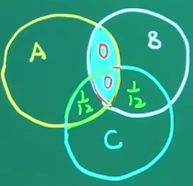
• 解 由于两直线相交, 故两直线的方向向量线性无关, 即 $\boldsymbol{\alpha}_1, \boldsymbol{\alpha}_2$ 线性无关,
• 分别取两直线上的点 $A\left(a_2, b_2, c_2\right), B\left(a_3, b_3, c_3\right)$, 则向量 $\overrightarrow{A B}$ 与两直线的方向向量是共面的,
  • 所以它们三者的混合积为 0 , 故
    • $\displaystyle \left|\begin{array}{lll}a_1 & a_2 & a_3-a_2 \\b_1 & b_2 & b_3-b_2 \\c_1 & c_2 & c_3-c_2\end{array}\right|=\left|\begin{array}{lll}a_1 & a_2 & a_3 \\b_1 & b_2 & b_3 \\c_1 & c_2 & c_3\end{array}\right|=0,$
    • 所以 $\boldsymbol{\alpha}_3$ 可由 $\boldsymbol{\alpha}_1, \boldsymbol{\alpha}_2$ 线性表示, 选 C.

(7)

设 $A, B, C$ 为三个随机事件, 且 $P(A)=P(B)=P(C)=\frac{1}{4}, P(A B)=0, P(A C)=P(B C)=$ $\frac{1}{12}$, 则 $A, B, C$ 中恰有一个事件发生的概率为 $(\quad)$
(A) $\frac{3}{4}$.
(B) $\frac{2}{3}$.
(C) $\frac{1}{2}$.
(D) $\frac{5}{12}$.

(7)

• 2025版

• 
  
• (1) 两个事件的加法公式:
  • $P(A \cup B)=P(A)+P(B)-P(A B)$
• (2) 三个事件的加法公式:
• $P\left(A_1 \cup A_2 \cup A_3\right)=P\left(A_1\right)+P\left(A_2\right)+P\left(A_3\right)-P\left(A_1 A_2\right)-P\left(A_1 A_3\right)-P\left(A_2 A_3\right)+P\left(A_1 A_2 A_3\right) .$
• 注意，" $A, B, C$ 中恰有一个发生"也可表示为 $A \cup B \cup C-A B \cup A C \cup B C$.
• $\text { 而 } P(A \cup B \cup C-A B \cup A C \cup B C)=P(A \cup B \cup C)-P(A B \cup A C \cup B C)$
  • 至少一个发生$\displaystyle \begin{array}{l}P(A \cup B \cup C)=P(A)+P(B)+P(C)-P(A B)-P(B C)-P(A C)+P(A B C) \\ =\frac{1}{4}+\frac{1}{4}+\frac{1}{4}-0-\frac{1}{12}-\frac{1}{12}+0=\frac{7}{12} .\end{array}$
  • 两个一起发生
    $\displaystyle P(A B \cup B C \cup A C) =P(A B)+P(B C)+P(A C)-P(A B C)-P(A B C)-P(A B C)+P(A B C)$
    • $P(A)+P(B)+P(C)-P(A B)-P(B C)-P(A C)_{+} P(A B C)$
    • $\displaystyle =0+\frac{1}{12}+\frac{1}{12}+0=\frac{1}{6}$
  • 三个同时发生$P(ABC)=0$
  • 至少一个发生的概率
    减去两个一起发生的概率
    再减去三个一起发生的概率
    只剩下只有一个发生的概率:$p=\frac{7}{12}-\frac{1}{6}=\frac{5}{12}$
• 定义三个事件 $A$, $B$, $C$ 的概率及它们之间的关系：
  • $P(A) = P(B) = P(C) = \frac{1}{4}$
  • $P(AB) = 0$（$A$ 和 $B$ 互斥），则$P(ABC)=0$
  • $P(AC) = P(BC) = \frac{1}{12}$

(8)

设 $X_{1}, X_{2}, \cdots, X_{100}$ 为来自总体 $X$ 的简单随机样本, 其中 $P\{X=0\}=P\{X=1\}=\frac{1}{2} . \Phi(x)$ 表 示标准正态分布函数, 则利用中心极限定理可得 $\displaystyle P\left\{\sum_{i=1}^{100} X_{i} \leqslant 55\right\}$ 的近似值为 $(\quad)$
(A) $1-\Phi(1)$.
(B) $\Phi(1)$.
(C) $1-\Phi(0.2)$.
(D) $\Phi(0.2)$.

(8)

• 由列维-林德伯格中心极限定理可知, 考虑独立同分布的随机变量 $X_1, X_2, \cdots, X_n, \cdots$. 若它们的期望为 $\mu$, 方差为 $\displaystyle \sigma^2$, 则当 $n$ 足够大时, 它们的和 $\displaystyle \sum_{k=1}^n X_k$ 近似服从正态分布 $\displaystyle N\left(n \mu, n \sigma^2\right)$.
• 解题过程
  • 由已知条件可知，样本容量 $n=100$.
  • 根据列维一林德伯格中心极限定理，
    $\displaystyle \sum_{i=1}^{100} X_i$ 近似服从均值为 $100 E(X)$ ，方差为 $100 D(X)$ 的正态分布.
  • 分别计算 $E(X), D(X)$.
• 计算 $E(X), D(X)$.
  • $\displaystyle E(X)=0 \times \frac{1}{2}+1 \times \frac{1}{2}=\frac{1}{2} .$
  • $\displaystyle E\left(X^2\right)=0^2 \times \frac{1}{2}+1^2 \times \frac{1}{2}=\frac{1}{2} .$
  • $\displaystyle D(X)=E\left(X^2\right)-[E(X)]^2=\frac{1}{2}-\frac{1}{4}=\frac{1}{4} .$
• 由题设, $E X=\frac{1}{2}, D X=\frac{1}{4}$, 且 $X_i$ 独立同分布, 则
  • $\displaystyle E\left(\sum_{i=1}^{100} X_i\right)=\sum_{i=1}^{100} E X_i=100 \times EX=100 \times \frac{1}{2}=50 ;$
  • $\displaystyle D\left(\sum_{i=1}^{100} X_i\right)=\sum_{i=1}^{100} D X_i=100 \times DX=100 \times \frac{1}{4}=25 .$
• 由独立同分布的中心极限定理可知
  • $\displaystyle \sum_{i=1}^{100} X_i$ 近似服从正态分布 $\displaystyle N(n \mu, n \sigma^2)\xlongequal[]{n=100}(50,25)$, 故
  • $\displaystyle P\left\{\sum_{i=1}^{100} X_i \leqslant 55\right\}\xlongequal[]{\text{标准化}}P\left\{\frac{\sum_{i=1}^{100} X_i-50}{5} \leqslant \frac{55-50}{5}\right\}=P\left\{\frac{\sum_{i=1}^{100} X_i-50}{5} \leqslant 1\right\} \approx \Phi(1) .$

二、填空题

(本题共 6 小题,每小题 4 分, 共 24 分, 把答案填在题中横线上.)

(9)

$\displaystyle \lim _{x \rightarrow 0}\left[\frac{1}{\mathrm{e}^{x}-1}-\frac{1}{\ln (1+x)}\right]=$

(9)

• 答 应填 -1
• $\displaystyle$原式$=\lim _{x \rightarrow 0} \frac{\ln (1+x)-\left(\mathrm{e}^x-1\right)}{\left(\mathrm{e}^x-1\right) \ln (1+x)}$
  • $\displaystyle \xlongequal[]{\text{化简分母}}\lim _{x \rightarrow 0} \frac{\ln (1+x)-\left(\mathrm{e}^x-1\right)}{x^2}$
• $\displaystyle \xlongequal[\text{或者洛必达两次}]{\text{分子用泰勒}}\lim _{x \rightarrow 0} \frac{x-\frac{1}{2} x^2+o\left(x^2\right)-\left[1+x+\frac{1}{2} x^2+o\left(x^2\right)-1\right]}{x^2}=-1 .$

(10)

设 $\displaystyle \left\{\begin{array}{l}x=\sqrt{t^{2}+1}, \\ y=\ln \left(t+\sqrt{t^{2}+1}\right),\end{array}\right.$ 则 $\left.\frac{\mathrm{d}^{2} y}{\mathrm{~d} x^{2}}\right|_{t=1}=$

(10)

• 答 应填 $-\sqrt{2}$.

高昆仑版

• $\displaystyle \frac{dy}{dx} \cdot \frac{y'_t}{x'_t} = \frac{\sqrt{1+t^2}}{t} \cdot \frac{1}{\sqrt{t^2+1}} = \frac{1}{t} .$
  • $\displaystyle \frac{d^2 y}{dx^2} = \left(\frac{1}{t}\right)' \cdot \frac{1}{x'_t} = -\frac{1}{t^2} \cdot \frac{1}{\sqrt{t^2+1}} \cdot \frac{t}{\sqrt{t^2+1}} = -\frac{\sqrt{t^2+1}}{t^3} .$
  • $\displaystyle \left. \frac{d^2 y}{dx^2} \right|_{t=1} = -\sqrt{2} .$

2024版

• 第一步：$\frac{dy}{dx} = \frac{\frac{dy}{dt}}{\frac{dx}{dt}}$
  • 计算 $\frac{dy}{dt}$
    • 应用求导公式：$\frac{dy}{dt} = \frac{1}{\sqrt{t^2+1}}$
      • 使用对数导数公式：$\left[\ln \left(x+\sqrt{x^2+1}\right)\right]'=\frac{1}{\sqrt{x^2+1}}$
      • 若不记得公式，详细计算：$\frac{dy}{dt} = \frac{\sqrt{t^2+1}+t}{\left(t+\sqrt{t^2+1}\right) \sqrt{t^2+1}} = \frac{1}{\sqrt{t^2+1}}$
  • 计算 $\frac{dx}{dt}$
    • 直接计算：$\frac{dx}{dt} = \frac{t}{\sqrt{t^2+1}}$
  • 最终结果：$\frac{dy}{dx} = \frac{1}{t}$
• 第二步：计算 $\frac{d^2 y}{dx^2} = \frac{d}{dx}\left(\frac{dy}{dx}\right) = \frac{\frac{d}{dt}\left(\frac{dy}{dx}\right)}{\frac{dx}{dt}}$
  • 求导：$\frac{d}{dt}\left(\frac{1}{t}\right) = -\frac{1}{t^2}$
  • 最终结果：$\frac{d^2 y}{dx^2} = -\frac{\sqrt{t^2+1}}{t^3}$
• 第三步：代入 $t = 1$ 并计算结果
  • 代入并计算：$\left.\frac{d^2 y}{dx^2}\right|_{t=1} = -\frac{\sqrt{1^2+1}}{1^3} = -\sqrt{2}$

(11)

若函数 $f(x)$ 满足 $f^{\prime \prime}(x)+a f^{\prime}(x)+f(x)=0(a>0), f(0)=m, f^{\prime}(0)=n$, 则 $\displaystyle \int_{0}^{+\infty} f(x) \mathrm{d} x=$

(11)

• 答 应填 $a m+n$.
• 解直接在微分方程 $\displaystyle f''(x) + a f'(x) + f(x) = 0$（$\displaystyle a > 0$）两端作积分
  • $\displaystyle \left. f'(x) \right|_0^{+\infty} + a f(x) \bigg|_0^{+\infty} + \int_0^{+\infty} f(x) \, dx = 0 .$
    • $\displaystyle f(+\infty) = \lim_{x \to +\infty} f(x) = 0$, $\displaystyle f'(+\infty) = \lim_{x \to +\infty} f'(x) = 0$，
    • $\displaystyle f(0)=m, f^{\prime}(0)=n$
  • 于是，$\displaystyle 0 - n + a(0 - m) + \int_0^{+\infty} f(x) \, dx = 0$。
    • 故 $\displaystyle \int_0^{+\infty} f(x) \, dx = a m + n$ .
• 为什么$\displaystyle f(+\infty) = \lim_{x \to +\infty} f(x) = 0$, $\displaystyle f'(+\infty) = \lim_{x \to +\infty} f'(x) = 0$，
  • 特征方程 $\displaystyle \lambda^2 + a\lambda + 1 = 0$，且注意到 $\displaystyle e^{-\infty} \to 0$。
    • 当 $\displaystyle 0 < a < 2$ 时，
      • $\displaystyle f(x) = e^{-\frac{a}{2}x} \left( C_1 \cos\left(\frac{\sqrt{4-a^2}}{2}x\right) + C_2 \sin\left(\frac{\sqrt{4-a^2}}{2}x\right) \right) .$
    • 当 $\displaystyle a = 2$ 时，$\displaystyle f(x) = (C_1 + C_2 x) e^{-x} .$
    • 当 $\displaystyle a > 2$ 时，$\displaystyle f(x) = C_1 e^{\frac{-a-\sqrt{a^2-4}}{2}x} + C_2 e^{\frac{-a+\sqrt{a^2-4}}{2}x} .$
• 解 直接在考场上有这种估计已经够用了,类似的问题读者还可以参考 2016 年的第(16) 题.

(12)

设函数 $\displaystyle f(x, y)=\int_{0}^{x y} \mathrm{e}^{xt^{2}} \mathrm{~d} t$, 则 $\left.\frac{\partial^{2} f}{\partial x \partial y}\right|_{(1,1)}=$

(12)

• 高昆仑版

• $\displaystyle \frac{\partial f}{\partial y} \left( e^{x(xy)^2} \cdot x \right)= x e^{x^3 y^2}$
• $\displaystyle \Rightarrow \frac{\partial^2 f}{\partial y \partial x} \xlongequal[\text{先}1\text{后}2]{\text{乘法求导}}e^{x^3 y^2} + x e^{x^3 y^2} \cdot 3 x^2 y^2 = e^{x^3 y^2} + 3 x^3 y^2 e^{x^3 y^2} .$
  • 因为 $\displaystyle \frac{\partial^2 f}{\partial y \partial x}$ 和 $\displaystyle \frac{\partial^2 f}{\partial x \partial y}$ 在点(1,1)都连续，
• $\displaystyle \left. \frac{\partial^2 f}{\partial x \partial y} \right|_{(1,1)} = \left. \frac{\partial^2 f}{\partial y \partial x} \right|_{(1,1)} = 4e .$

武忠祥版(先代后求)

  f
 / \ 
x   y

解
该问题涉及求函数 $\displaystyle f(x, y) = \int_{0}^{xy} \mathrm{e}^{xt^{2}} \mathrm{d} t$ 在点 (1,1) 的二阶混合偏导数 $\frac{\partial^{2} f}{\partial x \partial y}$。
计算具体点的混合偏导：可以用先带后求的思想

• 对x求完偏导以后,x就可以代入了
• 求函数 $f(x, y)$ 的偏导数。
  • 求 $f_y^{\prime}(x, y)$。
    • 对 $y$ 求偏导得：$f_y^{\prime}(x, y) = \mathrm{e}^{x(x y)^2} \cdot x=x \mathrm{e}^{x^3 y^2}$。
    • 先代后求 $f_y^{\prime}(x, 1)$。
      • 代入 $y = 1$，得到：$f_y^{\prime}(x, 1) = x \mathrm{e}^{x^3}$。
  • 求 $f_{yx}^{\prime\prime}(x, y)$。
    • 对$f_y^{\prime}(x, 1) = x \mathrm{e}^{x^3}$两边关于 $x$ 求偏导得：$f_{yx}^{\prime\prime}(x, y) = 1 \cdot e^{x^3}+x \cdot e^{x^3} \cdot 3 x^2\xlongequal[]{\text{代入}x=1}e+3 e=4 e$
    • 计算得到：$f_{yx}^{\prime\prime}(1, 1) = 4 \mathrm{e}$。
• 得到最终结果。
  • 在点 (1,1) 的二阶混合偏导数为 $4 \mathrm{e}$。

(13)

行列式 $\displaystyle \left|\begin{array}{cccc}a & 0 & -1 & 1 \\ 0 & a & 1 & -1 \\ -1 & 1 & a & 0 \\ 1 & -1 & 0 & a\end{array}\right|=$

(13)

• 答 应填 $a^2\left(a^2-4\right)$.
• 如果行列式每行元素之和相等, 都是 $s$, 则都可以按如下步脁操作
  • 第一步列变换：把其他列都加到第一列
  • 第二步行变换：其他行都减去第一行
  • 第三步展开：按第一列展开
• 每行元素之和相等
• 解 $\displaystyle \left|\begin{array}{cccc}a 0 -1 1 \\ 0 a 1 -1 \\ -1 1 a 0 \\ 1 -1 0 a\end{array}\right| \xlongequal[]{c2+c1}\left|\begin{array}{cccc}a a 0 0 \\ 0 a 1 -1 \\ 0 0 a a \\ 1 -1 0 a\end{array}\right|$
  • $\displaystyle \xlongequal[\text{有两列为}0]{\text{直接第一列展开}}a(-1)^{1+1}\left|\begin{array}{ccc}a 1 -1 \\ 0 a a \\ -1 0 a\end{array}\right|+(-1)^{4+1}\left|\begin{array}{ccc}a 0 0 \\ a 1 -1 \\ 0 a a\end{array}\right|$
  • $\displaystyle \xlongequal[\text{直接用对角线法则}]{\text{三阶行列式}}a^2\left(a^2-2\right)-2 a^2=a^2\left(a^2-4\right) .$
• 注 本题也可以将各行都加到第 1 行, 提出公因子 $a$, 再消零并展开.

(14)

设 $X$ 服从区间 $\left(-\frac{\pi}{2}, \frac{\pi}{2}\right)$ 上的均匀分布, $Y=\sin X$, 则 $\operatorname{Cov}(X, Y)=$

(14)

• • 确定 $X$ 的概率密度函数 $f(x)$
    • $X$ 服从区间 $\left(-\frac{\pi}{2}, \frac{\pi}{2}\right)$ 上的均匀分布，所以 $\displaystyle f(x) = \begin{cases}\frac{1}{\pi}, & x \in\left(-\frac{\pi}{2}, \frac{\pi}{2}\right), \\ 0, & \text{其他.}\end{cases}$
• 计算协方差 $\operatorname{Cov}(X, Y)$
  • $\operatorname{Cov}(X, Y)\xlongequal[]{Y=sinX}\operatorname{Cov}(X, \sin X)\xlongequal[]{=E(X Y)-E X \cdot E Y}E(X \sin X) - E(X) E(\sin X)$
    • 计算 $E(X \sin X)$:求谁的期望，就在它前面乘概率密度积分
      • 则期望
        $\displaystyle E(X \sin X) \xlongequal[]{\int_a^b x \cdot \sin x \cdot f(x) d x} \int_{-\frac{\pi}{2}}^{\frac{\pi}{2}} x \sin x \cdot \frac{1}{\pi} dx$
        • $\displaystyle \xlongequal[\text{区间对称，翻倍}]{\text{奇}\times\text{奇}=\text{偶}}\frac{2}{\pi} \int_0^{\frac{\pi}{2}} x \sin x dx$
        • $\displaystyle \xlongequal[]{\text{分布}}\underbrace{-\left.\frac{2}{\pi}\text{·} x \cos x\right|_0 ^{\frac{\pi}{2}}}_{=0}+\frac{2}{\pi}\text{·}\underbrace{ \int_0^{\frac{\pi}{2}} \cos x \mathrm{~d} x}_{=1}=\frac{2}{\pi}$
    • 计算 $E(X)$ 和 $E(\sin X)$
      • $\displaystyle E(X)\xlongequal[]{\frac{a+b}2}\frac{\frac{\pi}{2}+\left(-\frac{\pi}{2}\right)}{2}=0$
  • 合并计算结果:得出协方差
    • $\operatorname{Cov}(X, Y) = \frac{2}{\pi} - 0 \times 0 = \frac{2}{\pi}$

三、解答题

( 本题共 9 小题, 共 94 分, 解答应写出文字说明、证明过程或演算步骤.)

(15)

(本题满分 10 分)
求函数 $f(x, y)=x^{3}+8 y^{3}-x y$ 的极值.

(15)

2025版

• (1) 计算 $f(x, y)$ 的驻点.
• 解 $\displaystyle \left\{\begin{array}{l}f_x^{\prime}(x, y)=3 x^2-y=0, \\ f_y^{\prime}(x, y)=24 y^2-x=0 .\end{array}\right.$
  • 代入消元法 $\xrightarrow[]{y=3 x^2}24 y^2-x=0$
  • $\xrightarrow[]{24 \times 9 x^4-x=0}216 x^4=x\xrightarrow[]{x\left(216 x^3-1\right)=0}$
    • $x=0$ 或 $x=\frac{1}{6}$.
    • 由x的值解出y，于是, $\displaystyle \left\{\begin{array}{l}x=0, \\ y=0\end{array}\right.$ 或 $\displaystyle \left\{\begin{array}{l}x=\frac{1}{6}, \\ y=\frac{1}{12} .\end{array}\right.$
• 为了$AC-B^2$，求函数 $f(x, y)$ 在驻点的二阶偏导数
  • $A = f_{xx}^{\prime\prime}(x, y) \xlongequal[]{3x^2 - y\text{对}x\text{求导}} 6x$。
  • $B = f_{xy}^{\prime\prime}(x, y) \xlongequal[]{3x^2 - y\text{对}y\text{求导}} -1$
  • $C = f_{yy}^{\prime\prime}(x, y) \xlongequal[]{24y^2 - x\text{对}y\text{求导}} 48y$
• 用$AC-B^2$判断驻点是不是极值点
  • 考虑驻点 $(0,0)$.
    • $A=f_{x x}^{\prime \prime}(0,0)=0, \quad B=f_{x y}^{\prime \prime}(0,0)=-1, \quad C=f_{y y}^{\prime \prime}(0,0)=0 .$
      • $A C-B^2=0-1=-1<0$, 故点 $(0,0)$ 不是极值点.
  • 考虑驻点 $\left(\frac{1}{6}, \frac{1}{12}\right)$.
    • $A=f_{x x}^{\prime \prime}\left(\frac{1}{6}, \frac{1}{12}\right)=1, \quad B=f_{x y}^{\prime \prime}\left(\frac{1}{6}, \frac{1}{12}\right)=-1, \quad C=f_{y y}^{\prime \prime}\left(\frac{1}{6}, \frac{1}{12}\right)=4 .$
      • $A C-B^2=4-1=3>0$, 且 $A>0$, 故点 $\left(\frac{1}{6}, \frac{1}{12}\right)$ 为极小值点,
    • 极小值为$f\left(\frac{1}{6}, \frac{1}{12}\right)\xlongequal[]{f(x, y)=x^{3}+8 y^{3}-x y}\frac{1}{6^3}+\frac{8}{12^3}-\frac{1}{6 \times 12}=-\frac{1}{216} .$

(16)

(本题满分 10 分)
计算曲线积分 $I=\oint_{L} \frac{4 x-y}{4 x^{2}+y^{2}} \mathrm{~d} x+\frac{x+y}{4 x^{2}+y^{2}} \mathrm{~d} y$, 其中 $L$ 为 $x^{2}+y^{2}=2$, 方向为逆时针方向.

(16)

• 
  
• 拿到一个平面，如何选取方法，
  • 首先看积分曲线是否封闭，因为 $x^2+y^2=2$是一个圆心在原点的圆，所以封闭可以用格林公式
  • 但格林公式是有要求的，对于p和q
    • 被积函数在所围成的区域上要有连续一阶偏导
    • 所以分母$4x^2+y^2$不能为0
      被积函数存在分母,有奇异点(0,0)
• 构造辅助路径-做另一个封闭曲线：
  • 取 $L_1$ 为 $4x^2 + y^2 = 1$，方向为顺时针方向，相当于在里面做了一个椭圆。
    • 分母可以为1，也可以为任何一个常数
    • 里边为什么补顺时针？为了让它的正方向朝环形区域(沿着方向走的左侧是正方向)
  • 由 $L$ 和 $L_1$ 围成的平面区域记为 $D$。
• 在原曲线和辅助曲线中间的环形区域：应用格林公式：(沿着环形逆时针走左侧是正方向)
  • 将原积分分解为 $L + L_1$ 上的积分减去 $L_1$ 上的积分。
    • 对于 $L + L_1$ 上的积分，应用格林公式，将线积分转化为区域 $D$ 上的二重面积分。
      • 计算得到 $\iint_D \left[\frac{\partial}{\partial x}\left(\frac{x+y}{4x^2+y^2}\right)- \frac{\partial}{\partial y}\left(\frac{4x-y}{4x^2+y^2}\right)\right] dx dy$，结果为 0。
    • 计算 $L_1$ 上的积分：
      • 对于 $L_1$ 上的积分，转化为区域 $4x^2 + y^2 \leq 1$ 上的面积分,因分母为1，
        • 是封闭曲线，且分母不为零
        • 则可以使用格林公式
      • 则得到 $\iint_{4x^2+y^2 \leq 1} \left[\frac{\partial(x+y)}{\partial x}- \frac{\partial(4x-y)}{\partial y}\right] dx dy\text{＝}\iint_{4x^{2}+y^{2}\leq1}2dxdy$，结果为 $\pi$。
  • 合并结果：
    • 最终结果 $I =-\pi$。
• 类似的存在奇异点$(0\text{，}0)$的形式
  • $\displaystyle \int_{L}\frac{ydx-xdy}{x^2+y^2}$
  • $\displaystyle \int_{L}\frac{xdy-ydx}{x^2+y^2}$
  • $\displaystyle \int_{L}\frac{(x-y)dx+(x+y)dy}{(4x^2+y^2)^{3/2}}$这几个积分在做的时候
  • $\displaystyle \int_{L}\frac{(x+y)dx-(x-y)dy}{x^2+y^2}$
• 【例】计算曲线积分 $I=\oint_L \frac{x \mathrm{~d} y-y \mathrm{~d} x}{4 x^2+y^2}$, 其中 $L$ 是以点 $(1,0)$ 为中心, $R$ 为半径的圆周 $(R>1)$,取逆时针方向. (2000 年数学一试题)

(17)

设数列 $\left\{a_{n}\right\}$ 满足 $a_{1}=1,(n+1) a_{n+1}=\left(n+\frac{1}{2}\right) a_{n}$, 证明当 $|x|<1$ 时, 幂级数 $\displaystyle \sum_{n=1}^{\infty} a_{n} x^{n}$ 收玫, 并求其和函数.

(17)

• • 题目中给出了幂级数系数 $a_n$ 的递推关系式, 要求和函数, 可以利用已知关系构造微分方程, 通过解微分方程求得和函数.
• 解 计算幂级数的收敛半径 $R$.
  • 由 $(n+1) a_{n+1}=\left(n+\frac{1}{2}\right) a_n$
  • 可得, $\displaystyle \frac{a_n}{a_{n+1}}=\frac{n+1}{n+\frac{1}{2}}\xrightarrow[]{\text{求极限}}$
  • $\displaystyle R=\lim _{n \rightarrow \infty}\left|\frac{a_n}{a_{n+1}}\right|=\lim _{n \rightarrow \infty} \frac{n+1}{n+\frac{1}{2}}=1 .$
• 因此, 幂级数的收敛半径 $R=1$. 当 $|x|<1$ 时, 幂级数 $\displaystyle \sum_{n=1}^{\infty} a_n x^n$ 收敛.
• $\displaystyle S(x)=\sum_{n=1}^{\infty} a_n x^n$
• $\displaystyle S^{\prime}(x) =\sum_{n=1}^{\infty} na_n x^{n-1}\xlongequal[\text{内减外加}]{\text{内加外减}}\sum_{n=0}^{\infty} (n+1)a_{n+1} x^n$
  • $\displaystyle \xlongequal[a\text{从}1\text{开始}]{\text{拆项}}a_1+\sum_{n=1}^{\infty}(n+1) a_{n+1} x^n$
  • $\displaystyle \xlongequal[\text{级数转换思想}]{(n+1) a_{n+1}=\left(n+\frac{1}{2}\right) a_n} a_1+\sum_{n=1}^{\infty}\left(n+\frac{1}{2}\right) a_n x^n$
  • $\displaystyle \xlongequal[]{a_1=1}1+\sum_{n=1}^{\infty}\left(n+\frac{1}{2}\right) a_n x^n$
  • $\displaystyle \xlongequal[]{\text{去括号}}1+x \underbrace{\sum_{n=1}^{\infty} n a_n x^{n-1}}_{S^{\prime}(x)}+\frac{1}{2} \sum_{n=1}^{\infty} a_n x^n$
• 从而构造出关于$\displaystyle S^{\prime}(x)$的微分方程
  $\displaystyle S^{\prime}(x)=1+x S^{\prime}(x)+\frac{1}{2} S(x)$
• 解微分方程
  • $(1-x) S^{\prime}(x)-\frac{1}{2} S(x)=1$
  • $\displaystyle \xrightarrow[]{S(x)\text{替换成}y} y^{\prime}-\frac{1}{2(1-x)} y=\frac{1}{1-x}$
  • 用一阶线性微分方程求解
    $\displaystyle y=e^{\int \frac{1}{2(1-x)} d x}\left(\int \frac{1}{1-x} e^{-\int \frac{1}{2(1-x)} d x} d x+C\right)$
    • $\displaystyle y=\mathrm{e}^{-\int p(x) \mathrm{d} x}\left[\int Q(x) \mathrm{e}^{\int p(x) \mathrm{d} x} \mathrm{~d} x+C\right] .$
    • $\displaystyle e^{\int \frac{1}{2(1-x)} dx} = e^{-\frac{1}{2} \ln(1-x)}$
      • $\displaystyle = \left[ e^{\ln(1-x)} \right]^{-\frac{1}{2}}$
      • $\displaystyle = (1-x)^{-\frac{1}{2}}$
      • $\displaystyle = \frac{1}{\sqrt{1-x}}$
  • $\displaystyle \xlongequal[]{e^{\int \frac{1}{2(1-x)} d x}=\frac{1}{\sqrt{1-x}}}\frac{1}{\sqrt{1-x}}\left(\underline{\int \frac{1}{1-x} \cdot \sqrt{1-x} }d x+C\right)$
    • $\displaystyle \xlongequal[]{\text{整理}}\frac{1}{\sqrt{1-x}}\left(\int \frac{1}{\sqrt{1-x}} d x+C\right)$
    • $\displaystyle \xlongequal[\int \frac{1}{\sqrt{1-x}} d x=-2 \sqrt{1-x}]{\text{积分}}\frac{1}{\sqrt{1-x}}(-2 \sqrt{1-x}+C)$
    • $\displaystyle \xrightarrow[]{\text{整理}}y =-2+\frac{C}{\sqrt{1+x}}$
  • 当 $x=0$ 时, $y(0)=S(0)=0$,
    • $a_1 x+a_2 x^2+a_3 x^3+\cdots=S(x)$，则$\displaystyle S(0)=0$
    • 故 $0=-2+C$，解得 $C=2$.
  • 因此, $S(x)=\frac{2}{\sqrt{1-x}}-2, x \in(-1,1)$.

(18)

(本题满分 10 分)
设 $\displaystyle \Sigma$ 为曲面 $z=\sqrt{x^{2}+y^{2}}\left(1 \leqslant x^{2}+y^{2} \leqslant 4\right)$ 的下侧, $f(x)$ 是连续函数, 计算 $\displaystyle I=\iint_{\Sigma}[x f(x y)+2 x-y] \mathrm{d} y \mathrm{~d} z+[y f(x y)+2 y+x] \mathrm{d} z \mathrm{~d} x+[z f(x y)+z] \mathrm{d} x \mathrm{~d} y$.

(18)

• 分析 本题主要考査第二类曲面积分的计算.

• 本题中的被积函数含有抽象函数 $f$ ，可考虑利用两类曲面积分之间的联系消去该抽象函数。
  本题的典型错误：先补面再用高斯公式，

• 两类曲面积分之间的联系
  $\displaystyle \iint_{\Sigma} P \mathrm{~d} y \mathrm{~d} z+Q \mathrm{~d} z \mathrm{~d} x+R \mathrm{~d} x \mathrm{~d} y=\iint_{\Sigma}(P \cos \alpha+Q \cos \beta+R \cos \gamma) \mathrm{d} S,$

  • 其中 $\cos \alpha, \cos \beta, \cos \gamma$ 为有向曲面 $\displaystyle \Sigma$ 在点 $(x, y, z)$ 处的法向量的方向余弦.
  • 设有向曲面方程为 $z=z(x, y)$, 取上侧. 由于有向曲面 $\displaystyle \Sigma$ 取上侧
  • 公式推导: $\displaystyle$设$z=z(x, y)$，取上侧
    • $\displaystyle F(x, y, z)=0$，令 $F(x, y, z)=z-z(x, y)$
    • $\displaystyle \vec{n}=\left(F_x^{\prime}, F_y^{\prime}, F_z^{\prime}\right)=\left(-z_y^{\prime},-z_y^{\prime}, 1\right)$
    • 故 $\displaystyle \Sigma$ 的法向量的方向余弦为$\displaystyle \cos =\frac{\vec{n}}{\|\vec{n}\|}$
      $\displaystyle \cos \alpha=\frac{-z_x^{\prime}}{\sqrt{1+z_x^{\prime 2}+z_y^{\prime 2}}}, \quad \cos \beta=\frac{-z_y^{\prime}}{\sqrt{1+z_x^{\prime 2}+z_y^{\prime 2}}}, \quad \cos \gamma=\frac{1}{\sqrt{1+z_x^{\prime 2}+z_y^{\prime 2}}} .$

• 由于曲面 $\displaystyle \Sigma$ 取下侧，故 $\displaystyle \Sigma$ 的法向是 $n$ 与 $z$ 轴正向成钝角

• $F(x, y, z)=z-\sqrt{x^2+y^2}$

• 向上的法向量$\displaystyle \vec{n}=\left(F_x^{\prime}, F_y^{\prime}, F_z^{\prime}\right)=\left(-z_y^{\prime},-z_y^{\prime}, 1\right)$

  • 向下的法向量$n=\left(z_y^{\prime},z_y^{\prime}, -1\right) =\left(\frac{x}{\sqrt{x+y^2}}, \frac{y}{\sqrt{x+y^2}},-1\right)\xlongequal[]{z=\sqrt{x^{2}+y^{2}}}\left(\frac{x}{z}, \frac{y}{z},-1\right)$
    • $\displaystyle z=\sqrt{x^{2}+y^{2}}$
    • $\displaystyle z_x=\frac{x}{\sqrt{x^2+y^2}}=\frac{x}{z}$
    • $\displaystyle z_y=\frac{y}{\sqrt{x^2+y^2}}=\frac{y}{z}$

• $\displaystyle I=\iint_{\Sigma}[x f(x y)+2 x-y] \mathrm{d} y \mathrm{~d} z+[y f(x y)+2 y+x] \mathrm{d} z \mathrm{~d} x+[z f(x y)+z] \mathrm{d} x \mathrm{~d} y$

• $\displaystyle \iint_{\Sigma} =\iint_D\left(P z_x+Q z_y-R\right) d x d y$

  • $\displaystyle \left.=\iint_D\left[(x \cdot f+2 x-y) \frac{x}{z}+(y \cdot f+2 y+x) \frac{y}{z}-z f-z\right)\right] d x d y$
    • $\displaystyle \xlongequal[]{\text{合并同类项}}\iint_{\Sigma}\left[\left(\frac{x^2+y^2}{z}-z\right) f(x y)+\frac{2\left(x^2+y^2\right)}{z}-z\right] \mathrm{d} x \mathrm{~d} y$
    • $\displaystyle \xlongequal[]{\text{全打散拆开}}\frac{x^2}{z} f+\frac{2 x^2}{z}-\frac{x y}{z}+\frac{y^2}{z} f+\frac{2 y^2}{z}+\frac{x y}{z}-z \cdot f-z\xrightarrow[z^2=x^{2}+y^{2}]{\text{化简}}z$
  • $\displaystyle \iint_{\Sigma} z \mathrm{~d} x \mathrm{~d} y \xlongequal{\Sigma \text { 取下侧 }} \iint_D \sqrt{x^2+y^2} \mathrm{~d} x \mathrm{~d} y$
    • $\displaystyle \xlongequal[]{\text{极坐标}}\int_0^{2 \pi} \mathrm{~d} \theta \int_1^2 r^2 \mathrm{~d} r=\left.2 \pi \cdot \frac{r^3}{3}\right|_1 ^2=\frac{14 \pi}{3} .$

(19)

(本题满分 10 分)
设函数 $f(x)$ 在区间 $[0,2]$ 上具有连续导数, $f(0)=f(2)=0, M=\max _{x \in[0,2]}\{|f(x)|\}$. 证明:
( I ) 存在 $\xi \in(0,2)$, 使得 $\left|f^{\prime}(\xi)\right| \geqslant M$;
(II) 若对任意的 $x \in(0,2),\left|f^{\prime}(x)\right| \leqslant M$, 则 $M=0$.

(19)

• 证明 (I) 存在 $\xi \in(0,2)$ 使得 $\left|f^{\prime}(\xi)\right| \geqslant M$

• 设存在 $|f(c)|=M$
  • 若 $c=0$ 或 $2$
    • $f(x) \equiv 0$,由罗尔定理 $f^{\prime}(x)=0$, $x \in[0,2]$
  • 若 $c \in(0,1]$
    • 应用拉格朗日中值定理
      • 存在 $\xi \in(0, c)$，使 $f^{\prime}(\xi)=\frac{f(c)-f(0)}{c}$
      • 得 $\left|f^{\prime}(\xi)\right|=\frac{M}{c} \geqslant M$
  • 若 $c \in(1,2)$
    • 同理存在 $\xi \in(c, 2)$
      • $f^{\prime}(\xi)=\frac{f(2)-f(c)}{2-c}$
      • 得 $\left|f^{\prime}(\xi)\right|=\frac{M}{2-c} \geqslant M$

证明 (II) 若 $\left|f^{\prime}(x)\right| \leqslant M$ 则 $M=0$

• 提出假设 (反证法)
  • 假设 $M>0$
    • 则 $c \neq 0,2$
    • 分析 $c \in(0,1)$
      • 应用Newton-Leibniz公式
        • $\displaystyle M=|f(c)-f(0)|=\left|\int_0^c f^{\prime}(x) \mathrm{d} x\right|$
        • 得 $M \leqslant M c$，矛盾，故 $M=0$
    • 分析 $c \in(1,2)$
      • 类似地使用Newton-Leibniz公式
        • $\displaystyle M=|f(c)|=|f(2)-f(c)|=\left|\int_c^2 f^{\prime}(x) \mathrm{d} x\right|$
        • 得 $M \leqslant M(2-c)$，矛盾，故 $M=0$
    • 分析 $c=1$
      • 假设 $f(1)=M$，由费马引理得 $f^{\prime}(1)=0$
      • 设 $G(x)=f(x)-M x$，$0 \leqslant x \leqslant 1$
        • $G^{\prime}(x) \leqslant 0$，$G(x)$ 单调不增
        • $G(x) \equiv 0$，得 $f(x)=M x$
        • $f^{\prime}(1)=0$，得 $M=0$

(20)

(本题满分 11 分)
设二次型 $f\left(x_{1}, x_{2}\right)=x_{1}^{2}-4 x_{1} x_{2}+4 x_{2}^{2}$ 经正交变换 $\displaystyle \left(\begin{array}{l}x_{1} \\ x_{2}\end{array}\right)=\boldsymbol{Q}\left(\begin{array}{l}y_{1} \\ y_{2}\end{array}\right)$ 化为二次型 $g\left(y_{1}, y_{2}\right)=a y_{1}^{2}+4 y_{1} y_{2}+b y_{2}^{2}$, 其中 $a \geqslant b$.
(I) 求 $a, b$ 的值;
(II) 求正交矩阵 $Q$.

(20)

• (1) 由题意，二次型 $\displaystyle f(x_1, x_2)$ 与 $\displaystyle g(y_1, y_2)$ 的矩阵分别为

  • $\displaystyle A = \begin{pmatrix} 1 -2 \\ -2 4 \end{pmatrix}, \quad B = \begin{pmatrix} a 2 \\ 2 b \end{pmatrix},$

• $A$可以经过正交变换得到$B$

  • 于是 $\displaystyle A$ 与 $\displaystyle B$ 相似，所以 $\displaystyle$tr$(A) =$tr$(B)$，$\displaystyle |A| = |B|$，
    • 即$\displaystyle \begin{cases} a + b = 5, \\ ab - 4 = 0. \end{cases}$
  • 又 $\displaystyle a \geq b$，解得 $\displaystyle a = 4, b = 1$。

• 思路

  $$$$

  \begin{cases}
  \text{(1) 二次型 } & x^T A x \xrightarrow[]{\text{可逆 } x = C y} \text{ 二次型 } y^T B y
  \Rightarrow A \text{ 与 } B \text{ 合同，但不一定相似} \

  \text{计算思路}&\quad x^T A x \xrightarrow[]{\text{可逆 } x = C z} \text{同一标准型} \xleftarrow[]{\text{可逆 } y = C_2 z} y^T B y \
  &\Rightarrow C_1^T A C_1 = C_2^T B C_2 \rightarrow (C_1 C_2^{-1})T A (C_1 C_2^{-1}) = B \

  \

  \text{(2) 二次型 }& x^T A x \xrightarrow[]{\text{正交 } x = Q y} \text{ 二次型 } y^T B y
  \Rightarrow A \text{ 与 } B \text{ 合同且相似} \

  \text{计算思路} & \quad x^T A x \xrightarrow[]{\text{正交 } x = Q z} \text{同一标准型} \xleftarrow[]{\text{正交 } y = Q z} y^T B y \
  &\Rightarrow Q^T A Q = Q^T B Q \rightarrow (Q Q^{-1})T A (Q Q^{-1}) = B
  \end

  $$$$

• 由第( I ) 问可知, $\displaystyle \boldsymbol{A}=\left(\begin{array}{cc}1 & -2 \\ -2 & 4\end{array}\right), \boldsymbol{B}=\left(\begin{array}{ll}4 & 2 \\ 2 & 1\end{array}\right)$.

• 思路:$\displaystyle \left(Q_1 Q_2^{-1}\right)^{\top} A\left(Q_1 Q_2^{-1}\right)=B$

• 求A矩阵的特征值，求B矩阵的特征值(A和B相似)

  • $\displaystyle |A-\lambda E|=\left|\begin{array}{cc}1-\lambda & -2 \\ -2 & 4-\lambda\end{array}\right|=\lambda^2-5 \lambda+4-4=\lambda(\lambda-5)=0$
    • $\displaystyle \lambda_1=0 . \quad \lambda_2=5$
    • A和B相似，所以，B的特征值等于A的特征值

• 求A矩阵的特征向量，用来构造可逆矩阵$Q_1$

  • 计算A的属于特征值0的特征向量.
    • $\displaystyle \lambda=0 . \quad A x=0 . \quad\left(\begin{array}{cc}1 & -2 \\ -2 & 4\end{array}\right) \rightarrow\left(\begin{array}{cc}1 & -2 \\ 0 & 0\end{array}\right) \quad \alpha_1=\binom{2}{1}$
  • 计算A的属于特征值5的特征向量
    • $\displaystyle \lambda=5 . \quad(A-5 E) X=0 \quad\left(\begin{array}{ll}-4 & -2 \\ -2 & -1\end{array}\right) \rightarrow\left(\begin{array}{ll}2 & 1 \\ 0 & 0\end{array}\right) \quad \alpha_2=\binom{1}{-2}$
  • 对特征向量单位化
    $\displaystyle \gamma_1=\frac{1}{\sqrt{5}}\binom{2}{1} \quad \gamma_2=\frac{1}{\sqrt{5}}\binom{1}{-2}$
    • 因为是属于不同特征值的特征向量，所以天然正交
  • 经正交变换$\displaystyle x=Qz=\left(\begin{array}{cc}\frac{2}{\sqrt{5}} & \frac{1}{\sqrt{5}} \\ \frac{1}{\sqrt{5}} & \frac{-2}{\sqrt{5}}\end{array}\right) z .$
    • 使得$\displaystyle f \xrightarrow[]{\text{可化标准型}}5 z_2^2$

• 求B矩阵的特征向量，用来构造可逆矩阵$Q_2$

  • 计算B的属于特征值0的特征向量.
    • $\displaystyle \lambda=0 . \quad B x=0 \quad\left(\begin{array}{cc}4 2 \\2 1\end{array}\right) \rightarrow\left(\begin{array}{ll}2 1 \\0 0\end{array}\right) \quad \beta_1=\binom{1}{-2}$
  • 计算B的属于特征值5的特征向量.
    • $\displaystyle \lambda=5 \quad(B-5 E) x=0 \quad\left(\begin{array}{cc}-1 2 \\2 -4\end{array}\right) \rightarrow\left(\begin{array}{cc}1 -2 \\0 0\end{array}\right) \quad \beta_2=\binom{2}{1}$
  • 则有正交变换 $\displaystyle y=Q_2 z=\left(\begin{array}{cc}\frac{1}{5} \frac{2}{\sqrt{5}} \\-\frac{2}{\sqrt{5}} \frac{1}{\sqrt{5}}\end{array}\right) z .$
    • 使得$\displaystyle g \xrightarrow[]{\text{可化标准型为}} 5 z_2^2$

• $\displaystyle Q_1^{\top} A Q_1=\left(\begin{array}{ll}0 \\5\end{array}\right)=Q_2^{\top} B Q_2\xrightarrow[]{\text{从而}}Q_1^{\top} A Q_1=Q_2^{\top} B Q_2$

  • $\displaystyle \xrightarrow[]{\text{移项}}\left(Q_1 Q_2^{-1}\right)^{\top} A\left(Q_1 Q_2^{-1}\right)=B$

• $\displaystyle Q=Q_1 Q_2^{-1}\xlongequal[]{\text{正交}}Q_1 Q_2^{T}=\left(\begin{array}{cc}\frac{2}{\sqrt{5}} \frac{1}{\sqrt{5}} \\\frac{1}{\sqrt{5}} -\frac{2}{\sqrt{5}}\end{array}\right)\left(\begin{array}{cc}\frac{1}{\sqrt{5}} -\frac{2}{\sqrt{5}} \\\frac{2}{\sqrt{5}} \frac{1}{\sqrt{5}}\end{array}\right)=\left(\begin{array}{cc}\frac{4}{5} -\frac{3}{5} \\-\frac{3}{5} -\frac{4}{5}\end{array}\right)$

• 2015 年数一、数二、数三试题
  设矩阵 $\displaystyle \boldsymbol{A}=\left(\begin{array}{ccc}0 & 2 & -3 \\ -1 & 3 & -3 \\ 1 & -2 & a\end{array}\right)$ 相似于矩阵 $\displaystyle \boldsymbol{B}=\left(\begin{array}{ccc}1 & -2 & 0 \\ 0 & b & 0 \\ 0 & 3 & 1\end{array}\right)$.
  (I) 求 $a, b$ 的值; (II) 求可逆矩阵 $P$, 使 $P^{-1} A P$ 为对角矩阵.

• 2019 年数一、数二、数三试题
  已知矩阵 $\displaystyle \boldsymbol{A}=\left(\begin{array}{ccc}-2 & -2 & 1 \\ 2 & x & -2 \\ 0 & 0 & -2\end{array}\right)$ 与 $\displaystyle \boldsymbol{B}=\left(\begin{array}{ccc}2 & 1 & 0 \\ 0 & -1 & 0 \\ 0 & 0 & y\end{array}\right)$ 相似.
  (I) 求 $x, y$;
  (II) 求可逆矩阵 $P$, 使得 $P^{-1} A P=B$.

(21) (本题满分 11 分)

设 $\boldsymbol{A}$ 为 2 阶矩阵, $\boldsymbol{P}=(\boldsymbol{\alpha}, \boldsymbol{A} \boldsymbol{\alpha})$, 其中 $\boldsymbol{\alpha}$ 是非零向量且不是 $\boldsymbol{A}$ 的特征向量.
( I ) 证明 $\boldsymbol{P}$ 为可逆矩阵;
(II) 若 $\boldsymbol{A}^{2} \boldsymbol{\alpha}+\boldsymbol{A} \boldsymbol{\alpha}-6 \boldsymbol{\alpha}=\mathbf{0}$, 求 $\boldsymbol{P}^{-1} \boldsymbol{A P}$, 并判断 $\boldsymbol{A}$ 是否相似于对角矩阵.

(21)

• • 反证法
    • 若 $\displaystyle P$ 不可逆，$\displaystyle |\alpha, A\alpha| = 0 \Rightarrow \alpha$ 与 $\displaystyle A\alpha$ 相关 $\displaystyle \Rightarrow \alpha$，$\displaystyle A\alpha$ 成比例
      • 则 $\displaystyle \exists k$，使 $\displaystyle A\alpha = k\alpha$，说明 $\displaystyle \alpha$ 为 $\displaystyle A$ 对应于 $\displaystyle \lambda = k$ 的特征向量，与题中条件相悖
        • 题中条件:其中 $\boldsymbol{\alpha}$ 是非零向量且不是 $\boldsymbol{A}$ 的特征向量.
• $\displaystyle \therefore P$可逆
  (II) 若 $\boldsymbol{A}^{2} \boldsymbol{\alpha}+\boldsymbol{A} \boldsymbol{\alpha}-6 \boldsymbol{\alpha}=\mathbf{0}$, 求 $\boldsymbol{P}^{-1} \boldsymbol{A P}$, 并判断 $\boldsymbol{A}$ 是否相似于对角矩阵.
• $\displaystyle$设$P_{}^{-1} A P=B \xrightarrow[]{\text{左乘}P} A P=P B$
  • $\displaystyle A(\alpha \cdot A \alpha)=(\alpha \cdot A \alpha) B .$
  • $\displaystyle \xrightarrow[]{\boldsymbol{P}=(\boldsymbol{\alpha}, \boldsymbol{A} \boldsymbol{\alpha})}(\alpha \cdot A \alpha) B=\left(A \alpha \cdot A^2 \alpha\right)$
    • $\displaystyle \xrightarrow[]{\boldsymbol{A}^{2} \boldsymbol{\alpha}+\boldsymbol{A} \boldsymbol{\alpha}-6 \boldsymbol{\alpha}=\mathbf{0}}(A \alpha$，$6\alpha-A \alpha)$
    • $\displaystyle (\alpha \cdot A \alpha)B=(A \alpha$，$6 \alpha-A \alpha)$
      • $\displaystyle (\alpha \cdot A \alpha)\left(\begin{array}{cc}0 6 \\1 -1\end{array}\right)=(A \alpha$，$6 \alpha-A \alpha)$
• 求得B的系数矩阵
  $\displaystyle B=\left(\begin{array}{cc}0 & 6 \\ 1 & -1\end{array}\right)=P^{-1} A P$
  • 因为A和B相似，所以A和B的特征值一样
  • 求B的特征值
    • 则有 $\displaystyle |\lambda \boldsymbol{E}-\boldsymbol{B}|=\left|\begin{array}{cc}\lambda & -6 \\ -1 & \lambda+1\end{array}\right|=\lambda^2+\lambda-6=(\lambda-2)(\lambda+3)$,
      • 得 $\boldsymbol{B}$ 的特征值为 $2,-3$.
  • $A$有两个不同的特征值
    • 所以 $\boldsymbol{A}$ 相似于对角矩阵 $\displaystyle \left(\begin{array}{cc}2 & 0 \\ 0 & -3\end{array}\right)$.

解法2

• $\displaystyle \boldsymbol{A P}\xlongequal[]{\boldsymbol{P}=(\boldsymbol{\alpha}, \boldsymbol{A} \boldsymbol{\alpha})}\left(\boldsymbol{A} \boldsymbol{\alpha}, \boldsymbol{A}^2 \boldsymbol{\alpha}\right)\xlongequal[]{\boldsymbol{A}^{2} \boldsymbol{\alpha}+\boldsymbol{A} \boldsymbol{\alpha}-6 \boldsymbol{\alpha}=\mathbf{0}}(\boldsymbol{A \alpha}, 6 \boldsymbol{\alpha}-\boldsymbol{A \alpha})=(\boldsymbol{\alpha}, \boldsymbol{A} \boldsymbol{\alpha})\left(\begin{array}{cc}0 & 6 \\1 & -1\end{array}\right)=\boldsymbol{P}\left(\begin{array}{cc}0 & 6 \\1 & -1\end{array}\right),$
• 所以$\displaystyle \boldsymbol{P}^{-1} \boldsymbol{A P}=\left(\begin{array}{cc}0 & 6 \\1 & -1\end{array}\right),$可知矩阵 $\boldsymbol{A}$ 与 $\displaystyle \left(\begin{array}{cc}0 & 6 \\ 1 & -1\end{array}\right)$ 相似,

(22)

(本题满分 11 分)
设随机变量 $X_{1}, X_{2}, X_{3}$ 相互独立, 其中 $X_{1}$ 与 $X_{2}$ 均服从标准正态分布, $X_{3}$ 的概率分布为 $P\left\{X_{3}=0\right\}$

• $=P\left\{X_{3}=1\right\}=\frac{1}{2} \cdot Y=X_{3} X_{1}+\left(1-X_{3}\right) X_{2}$.
  (I ) 求二维随机变量 $\left(X_{1}, Y\right)$ 的分布函数,结果用标准正态分布函数 $\Phi(x)$ 表示;
  (II) 证明随机变量 $Y$ 服从标准正态分布.

(22)

解

• 全集分解∶一个离散，一个连续
  • 2020年第22题，2019年第22题，2017年第22题，2016年第22题，2014年第22题
  • 全集分解的思想∶A的发生伴随着其他几个事件的发生图示
    • 1
    • $P(A)=P\left(A B_1\right)+P\left(A B_2\right)+P\left(A B_3\right)$
• 先要会写二维随机变量$(X,Y)$的分布函数的定义$F(x, y)=P\{X\leq x, Y \leq y\}$
  • 分析题目中的条件
    • $X_1, X_2$ 均服从标准正态分布∶$X_1, X_2 \sim N(0,1)$,
    • $X_3$ 的概率分布0，1分布为 $P\left\{X_3=0\right\}\text{，}P\left\{X_3=1\right\}=\frac{1}{2}$
      • 则$\displaystyle X_3 \sim\left(\begin{array}{cc}0 & 1 \\ \frac{1}{2} & \frac{1}{2}\end{array}\right)$
• 把Y给换掉∶$=P\{X_1 \leqslant x, \underbrace{X_3 X_1+\left(1-X_3\right) X_2 \leqslant y}_{\text{全集分解}}\}$
  • 对离散的进行全集分解(也就是全概率公式的应用)
    只要这里边有离散的随机变量，就对离散的进行分解
    • $X_3$是离散的，对它进行全集分解。
      $=\underbrace{P\left\{X_1 \leqslant x, Y \leqslant y, X_3=0\right\}}_{\text{当}X_{3}=0\text{时，}Y=X_{2}}+\underbrace{P\left\{X_1 \leq x\right.,\left.Y \leqslant y,X_3=1\right\}}_{\text{当}X_{3}=1\text{时，}Y=X_{1}}$
    • 将$X_3$代入题中所给公式$Y=X_3 X_1+\left(1-X_3\right) X_2$，分别得到
      • 当$X_{3}=0$时，$Y=X_{2}$
      • 当$X_{3}=1$时，$Y=X_{1}$
      • 从而将$Y$换成对应情况的的$X$，得$=P\underbrace{\left\{X_1 \leq x, X_2 \leq y\text{，}X_3=0\right\}}_{\Phi(x) \cdot \Phi(y) \text{·}\frac12}+\underbrace{\\P\left\{X_1 \leq x, X_1 \leq y, X_3=1\right\}}_{\Phi(\min \{x, y\})\text{·}\frac12}$
• 化简环节
  • 由随机变量 $X_1, X_2, X_3$ 相互独立，将乘积的概率化为概率的乘积
    只有拆开才能继续进行概率的计算
    • 拆第一部分∶$P\left\{X_1 \leq x\right\}\text{·} P\left\{X_2 \leqslant y\right\} .P\left\{X_3=0\right\}$
    • 拆第二部分∶$P\left\{X_1 \leqslant x, X_{21}\leqslant y\right\}$合并为$P\left\{X_1 \leq \min (x, y)\right\}$
      整体写成$P\left\{X_1 \leq \min (x, y)\right\} \cdot P\left\{X_3=1\right\}$
  • 写出对应分布函数，由$X_1, X_2$ 均服从标准正态分布，则
    • $P\left\{X_1 \leq x\right\}\text{·} P\left\{X_2 \leqslant y\right\} .P\left\{X_3=0\right\}$＝$\Phi(x) \cdot \Phi(y) \cdot \frac{1}{2}$
    • $P\left\{X_1 \leq \min (x, y)\right\} \cdot P\left\{X_3=1\right\}$＝$\Phi(\min \{x, y\}) \cdot \frac{1}{2}$
• 关键∶全概率体现为∶对离散型进行全集分解
• II) 证时随机变量 $Y$ 服从标准正态分布
  • 已知二维的联合分布 $F(x, y) \rightarrow\text{求一维的边缘分布} F_Y(y)$
    • 令$x\rightarrow+\infty$，$y$不动
    • $F_Y(y)=F^{\prime}(+\infty, y)=\frac{1}{2} \Phi(+\infty) \text{·}\Phi(y)+\frac{1}{2} \Phi(y)$
      • 由$\Phi(+\infty)=1$
      • 化简得，$\frac{1}{2} \cdot \Phi(y) \cdot 1+\frac{1}{2} \Phi(y)=\Phi(y)$
  • 从而证得$Y$服从标准正态分布
• 有意识的带你如何思考(一道题拿到手的思考方式)
  • 第一步∶是不是我自己把这个分布函数给它写出来啊？
    • 那有同学说，哎呀，我这不敢用这小x小y
    • 就这随便你写个u，v啊都行，没有人管你这个自变量字母，都无所谓哈
  • 下一步∶在我们要求$Y\leq y$的题目中，是不是$Y$会换成$X$的函数对吧？
    • 就要用已知推未知，那么这里的$Y$你肯定要自然的想到我换成它的表达式。他表达式给你不就是为了换吗？是不是？
    • 这是这一步，我们为什么能想得到下一步呢？
  • 第三步为什么想得到呢？
    • 因为我看到里面有离散型了，而我们在20年之前做过很多，只要这个里面有离散型，我就对离散的变量进行全集分解
      • 因为有离散，也有连续是吧？
      • X1X2是连续型，那么离散和连续的掺杂在一起，我是不是就要对离散全局分解？所以我很自然的往这一步尝试
        • 但是这一步，它就是一个有点忐忑的尝试，因为确实可能之前没做过这个题，
        • 但是你就打开试嘛，一打开发现诶，很顺，我后面的步骤都带进去了，那么这个尝试就就成功了
  • 我们做题就是不可能都站在上帝视角，
    • 同学们第一步肯定这样做，第二步肯定这样做，不可能都
    • 我是试出来的，当然是要结合过往的经验
  • 就我今天会给你去带这个感觉好吗？就今天讲的比较快，你能体会多少算多少哈，因为咱是空降到一个难点，这个没办法那

(23)

(本题满分 11 分)
设某种元件的使用寿命 $T$ 的分布函数为

• $\displaystyle F(t)= \begin{cases}1-\mathrm{e}^{-\left(\frac{t}{\theta}\right)^{\mathrm{m}}}, & t \geqslant 0, \\ 0, & \text { 其他, }\end{cases}$
  其中 $\theta, m$ 为参数且大于零.
  ( I ) 求概率 $P\{T>t\}$ 与 $P\{T>s+t \mid T>s\}$, 其中 $s>0, t>0$.
  (II) 任取 $n$ 个这种元件做寿命试验, 测得它们的寿命分别为 $t_{1}, t_{2}, \cdots, t_{n}$. 若 $m$ 已知, 求 $\theta$ 的最 大似然估计值 $\hat{\theta}$.

(23)

• • (1) 由条件知
    • $\displaystyle P\{T > t\} = 1 - P\{T \leq t\}$
      • $\displaystyle = 1 - F(t) =1-\left[1-e^{-\left(\frac{t}{\theta}\right)^m}\right]= e^{-\left(\frac{t}{\theta}\right)^m} .$
    • $\displaystyle P\{T > s+t \mid T > s\} = \frac{P\{T > s+t, T > s\}}{P\{T > s\}} \xlongequal[]{\text{取交集}}\frac{P\{T > s+t\}}{P\{T > s\}}$
      • $\displaystyle =\frac{e^{-\left(\frac{s+t}{\theta}\right)^m}}{e^{-\left(\frac{s}{\theta}\right)^m}} \xlongequal[]{\text{指数相减}}e^{\left(\frac{s}{\theta}\right)^m-\left(\frac{s+t}{\theta}\right)^m}$
        • 其中$\displaystyle P\{T > s+t\}\xlongequal[]{\text{类比}T\text{＞}s\text{的概率}}e^{-\left(\frac{s+t}{\theta}\right)^m}$
• ( II) 分布函数求导得概率密度 $f(t ; \theta)$.
  $\displaystyle f(t ; \theta)=F^{\prime}(t ; \theta)=\left\{\begin{array}{ll} -\mathrm{e}^{-\left(\frac{1}{\theta}\right)^m} \cdot(-m) \cdot\left(\frac{t}{\theta}\right)^{m-1} \cdot \frac{1}{\theta}, & t>0, \\ 0, & \text { 其他 } \end{array}\right.$
  • $\displaystyle \begin{aligned}\xlongequal[]{\text{整理}} \begin{cases}\frac{m t^{m-1}}{\theta^m} \mathrm{e}^{-\left(\frac{t}{\theta}\right)^m,}, & t>0, \\ 0, & \text { 其他. }\end{cases}\end{aligned}$
• 连续型:用概率密度连乘构造似然函数
  $\displaystyle L(\theta) = f(t_1) \cdot f(t_2) \cdots \cdot f(t_n)$
  • $\displaystyle = \frac{m t_1^{m-1}}{\theta^m} e^{-(\frac{t_1}{\theta})^m} \cdot \frac{m t_2^{m-1}}{\theta^m} e^{-(\frac{t_2}{\theta})^m} \cdots \cdot \frac{m t_n^{m-1}}{\theta^m} e^{-(\frac{t_n}{\theta})^m}$
  • $\displaystyle \xlongequal[]{\text{合并同类项}}m^n \cdot \theta^{-mn} \cdot (t_1 t_2 \cdots t_n)^{m-1} e^{-\frac{1}{\theta^m} \left[ \sum_{i=1}^{n} t_i^m \right]}$
• 取对数:为了方便求导，
  $\displaystyle \ln L(\theta) = n \ln m - mn \ln \theta + (m-1) \ln (t_1 \cdots t_n) - \frac{1}{\theta^m} \sum_{i=1}^{n} t_i^m$
• 对$\theta$求导，求驻点(可能的极值点)
  $\displaystyle \frac{d \ln L(\theta)}{d\theta} = -\frac{mn}{\theta} + \frac{m}{\theta^{m+1}} \sum_{i=1}^{n} t_i^m = 0$
  • $\displaystyle \xrightarrow[]{\text{同乘} \theta\text{，移项}} \theta = \sqrt[m]{\frac{1}{n} \sum_{i=1}^{n} t_i^m}$
• 最终结果:$\displaystyle \hat{\theta}=\sqrt[m]{\frac{1}{n} \sum_{i=1}^n t_i^m}$